Driving an Autonomous Vehicle in a 3D Simulation Environment with Recorded Synthetic Data

With advancements in the automotive industry, various student competitions have introduced the driverless category, where the goal of the teams is to design and build an autonomous vehicle that can compete in different disciplines.

Using MATLAB and Simulink, you can design automated driving system functionality including sensing, path planning, sensor fusion and control systems.

In this article, we will demonstrate an approach to drive an autonomous vehicle in a closed-loop circuit. The task here is to drive the car in an unknown environment avoiding collision with the cones ensuring to complete the necessary laps.

 

Scene Creation

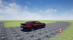
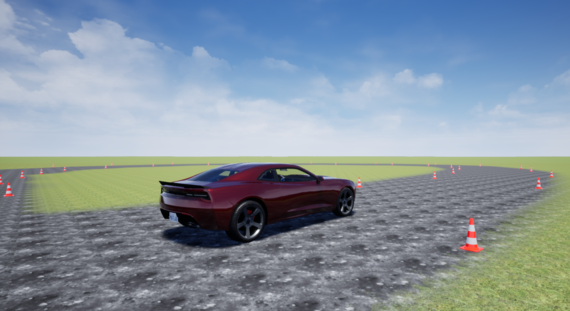
The first step is to create a 3D simulation environment consisting of a vehicle, track, and cones. The Vehicle Dynamics Blockset Toolbox comes installed with prebuilt 3D scenes to simulate and visualize the vehicles modeled in Simulink. These 3D scenes are visualized using the Unreal Engine from Epic Games.

Fig 1. Custom scene in Unreal

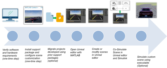
As the current problem requires a customized scene, we used the Unreal Editor and the Vehicle Dynamics Blockset Interface for Unreal Engine 4 Projects support package to build the scene. To learn how to customize scenes (Figure 2), please follow the steps explained in the documentation.

 

Fig 2. Steps for creating custom scene

 

 

Lap1: Environment Mapping

The next task is to map the environment. As mentioned in the previous section, the driverless vehicle is in an unknown environment that consists of cones kept on both sides of the track. To detect the cones and generate a reference path for the first lap, we have built a Simulink model as shown in Figure 3.

Fig 3. Simulink model for environment mapping

 

Figure 4 shows the steps performed by the model in the first lap:

Fig 4. Block diagram representation of environment mapping

 

Lidar mounting: The purpose of the lidar is to measure the distance to the cones. The Simulation 3D Lidar block provides an interface to the lidar sensor in a 3D simulation environment. The environment is rendered using the Unreal Engine from Epic Games. The block returns a point cloud with the specified field of view and angular resolution.

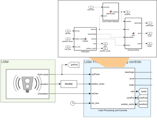
Fig 5. Lidar processing and controls

Cone detection: The goal of the cone detection algorithm is to cluster all points that belong to one cone and identify the position of the cones. This is done by calculating the distance between consecutive points in the point cloud. The points that belong to the same cone are close to each other, while cones are relatively far apart from each other. After clustering, the midpoint of the cone is the mean of the position of all the points in the cone.

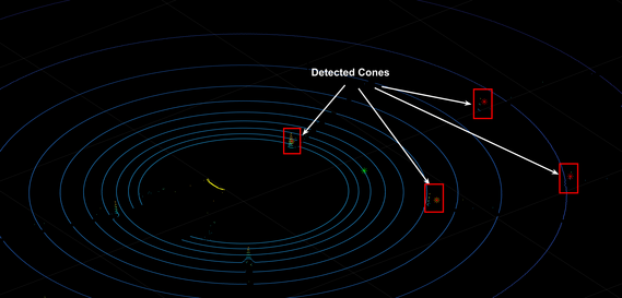
Fig 6. Plot showing cones detected in the point cloud

Driver controls

• Identify the two most significant cones in front of the vehicle
• Avoid crashing into any of the cones

This is done by finding the two closest cones and calculating the midpoint of those cones. The algorithm generates acceleration, steering commands towards this midpoint. The algorithm also limits the maximum speed of the vehicle to a pre-set threshold.

Vehicle dynamics: The vehicle dynamics model (Figure 7) consists of a vehicle body, simplified powertrain, driveline, longitudinal wheel, and kinematic steering. The purpose of the model is to calculate the position and orientation of the vehicle based on the steering, acceleration, and deceleration commands. To learn how to simulate longitudinal and lateral vehicle dynamics, refer to this video. The Simulation 3D Vehicle with Ground Following block and the Simulation 3D Scene Configuration block is used for setting up the 3D simulation environment in the Unreal Engine.

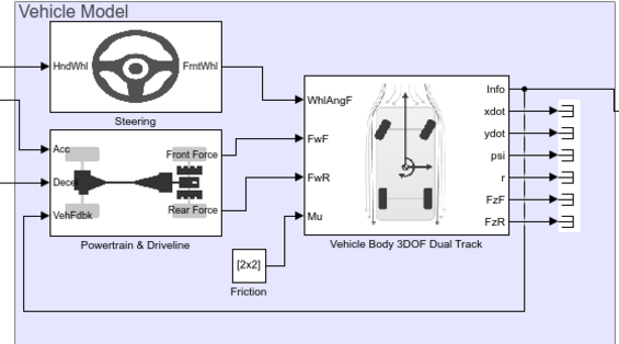
Fig 7. Vehicle model

Output: Once we run the simulation, the lidar successfully detects the cones. Further, the vehicle maps the environment and generates a reference trajectory. However, the vehicle moves slowly at a maximum velocity of 8 m/s.

 

Lap2: Reference trajectory tracking

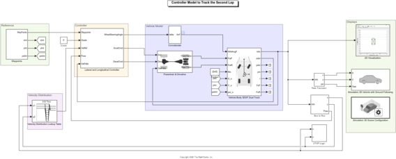
In the second lap, the vehicle tracks a reference path obtained from the first lap simulation. Figure 8 shows the Simulink model. Compared to the last model, in this model, we have removed the lidar block and have added the longitudinal and lateral controllers.

Fig 8. Simulink model for reference trajectory tracking

Now, it's a classical closed-loop control system problem where the controller's task is to output the required steering command, acceleration command, and deceleration command to track the reference path with a higher velocity.

Figure 9. Closed-loop block diagram for second lap

Lateral controller: Pure pursuit controller has been used for lateral control of the vehicle. To implement the controller in Simulink we have used a Pure Pursuit block to measure the target direction. Further, the target direction is converted into the required steering angle using wheel steering angle formulation. To learn more about vehicle path tracking using a pure pursuit controller, please refer to this video.

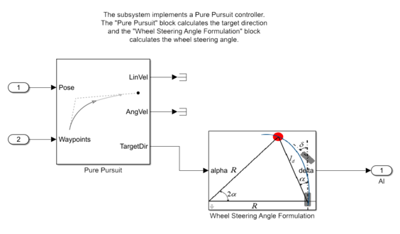
Figure 10. Pure pursuit controller

Longitudinal controller: The Longitudinal Driver block is used to regulate the speed of the vehicle. Specifically, it is a PI controller that generates the actuator signal for the reference speed.

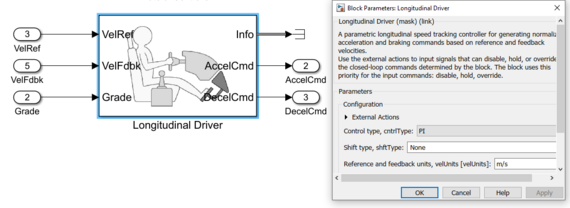
Figure 11. Longitudinal driver

Please note that currently, we have simplified the procedure of developing a speed profile by using a lookup table to define velocities at different regions. However, recommendation would be to use the Velocity Profiler block to automate the process of velocity profile generation.

Result: Figure 12 shows the comparison of the simulated trajectory and the reference trajectory. It is evident from the results that the lateral controller successfully tracks the reference path. In addition to the lateral control action, the longitudinal driver is able to regulate the desired velocity.

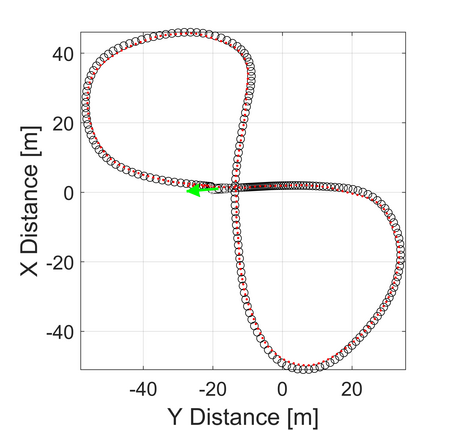
Fig 12. Vehicle trajectory obtained in second lap

Summary

The article showed how MathWorks tools can be used for driving a vehicle autonomously on a closed-loop track in presence of obstacles. You can extend this approach and leverage the examples provided in the documentation to design and simulate your autonomous vehicle.

 

Contact Us

Please feel free to reach out to us at racinglounge(at)mathworks.com in case of any queries. Also, join our MATLAB and Simulink Racing Lounge Facebook group for the latest technical articles, videos, and upcoming live sessions.

---